目标检测 | 目标检测综述

思维导图

• 目标检测综述
  • 定义
  • 存在的挑战
  • 目标检测发展历程
  • 传统目标检测算法
  • 深度学习的目标检测算法
  • 深度学习的优势
    • 传统机器视觉的局限
    • 深度学习算法的独特优势
  • RCNN 系列
    • RCNN
    • Fast-RCNN
    • Faster-RCNN
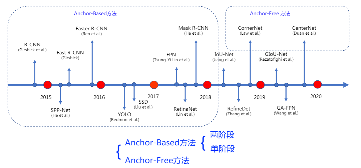
  • Anchor 和 Anchor-Based 方法
    • 两阶段方法
    • 一阶段方法
    • Anchor 缺点
  • Anchor-Free 方法
    • 基于关键点的检测算法
    • 基于中心的检测算法
  • 三种算法对比
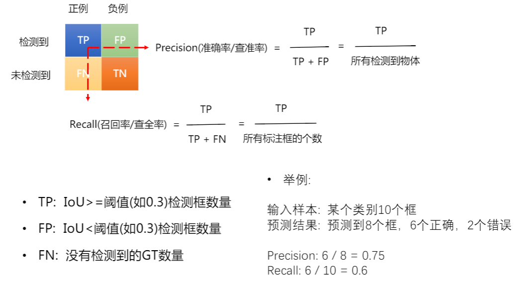
  • 基本术语
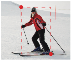
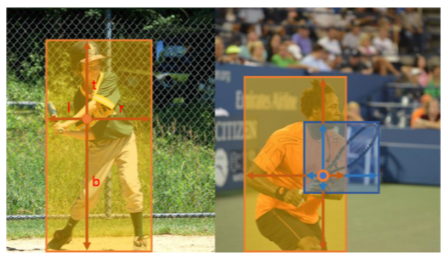
    • BBox
    • Anchor
    • RoI
    • Region Proposal
    • RPN
    • IoU
    • mAP
    • NMS[^3][4]
  • 常用开源数据集

学习资料

• PaddlePaddle
• 大话目标检测经典模型（RCNN、Fast RCNN、Faster RCNN）
• 《目标检测手把手入门教程》中的《Backbone与Detection head》 作者：Kissrabbit（知乎）

定义^[1]

目标检测，也叫目标提取，是一种基于目标几何和统计特征的图像分割。它将目标的分割和识别合二为一，其准确性和实时性是整个系统的一项重要能力。
它将目标的分割和识别合二为一，其准确性和实时性是整个系统的一项重要能力。尤其是在复杂场景中，需要对多个目标进行实时处理时，目标自动提取和识别就显得特别重要。
随着计算机技术的发展和计算机视觉原理的广泛应用，利用计算机图像处理技术对目标进行实时跟踪研究越来越热门，对目标进行动态实时跟踪定位在智能化交通系统、智能监控系统、军事目标检测及医学导航手术中手术器械定位等方面具有广泛的应用价值。

存在的挑战

• 环境影响
• 模糊
• 密集 crowded
• 遮挡 occluded
• 重叠 highly overlapped
• 多尺度
  • 小目标 extremely small
  • 大目标 very large
• 小样本
• 旋转框
• 体积、功耗、实时性
• ……

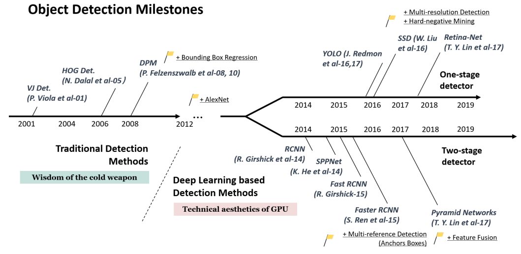
目标检测发展历程^[2]

传统目标检测算法

digraph G{
    node [shape=box width=3]
    a [label="区域选择\n（滑动窗口）" ]
    b [label="提取特征\n（SIFT、HOG）"]
    c [label="分类\n（SVM、Adaboost）"]
    d [label="后处理\n（NMS：过滤框）"]

    a->b
    b->c
    c->d
}

深度学习的目标检测算法

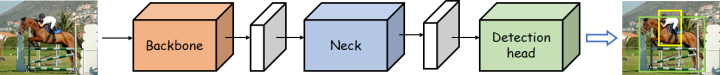
Backbone network，即主干网络，是目标检测网络最为核心的部分，大多数时候，backbone选择的好坏，对检测性能影响是十分巨大的。通常，为了实现从图像中检测目标的位置和类别，我们会先从图像中提取出些必要的特征信息，比如HOG特征，然后利用这些特征去实现定位和分类。而在深度学习这一块，这一任务就交由backbone网络来完成。深度学习的强大之处就在于其特征提取的能力，在很多任务上都超越了人工特征。
当然，这里提出的是什么样的特征，我们是无从得知的，毕竟深度学习的“黑盒子”特性至今还无法真正将其面纱揭开。
从某种意义上来说，如何设计好的backbone，更好地从图像中提取信息，是至关重要的，因为特征提取不好，自然会影响到后续的定位检测。

Neck network，即颈部网络，Neck部分的主要作用就是将由backbone输出的特征进行整合。其整合方式有很多，最为常见的就是FPN（Feature Pyramid Network）。除了FPN，还有SPP模块，这也是很常用的一个Neck结构。除此之外，还有：

1. RFB：出自《Receptive Field Block Net for Accurate and Fast Object Detection》

2. ASPP：出自《DeepLab: Semantic image segmentation with deep convolutional nets, atrous convolution, and fully connected CRFs》

3. SAM：出自《CBAM: Convolutional block attention module》

4. PAN：出自《Path aggregation network for instance segmentation》。PAN是一个非常好用的特征融合方式，在FPN的bottom-up基础上又引入了top-down二次融合，有效地提升了模型性能。

Detection head，即检测头，这一部分的作用就没什么特殊的含义了，就是若干卷积层进行预测，也有些工作里把head部分称为decoder（解码器）的，这种称呼不无道理，head部分就是在由前面网络输出的特征上去进行预测，约等于是从这些信息里解耦出来图像中物体的类别和位置信息。

深度学习的优势

传统机器视觉的局限

• 模板匹配误报高
  • 因为待识别目标（缺陷）千变万化
• 算法适应性差
  • 因为不同产线、产品、微细差别需重复开发
• 解决问题有限
  • 因为复杂背景、纹理难处理
• 开发、维护成本巨大
  • 因为新缺陷、新Trick意味着新补丁

深度学习算法的独特优势

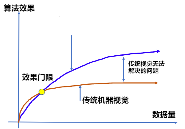
• 算法适应性强
• 更好的平衡精度&过检率
• 可迁移学习，经验复用

RCNN 系列

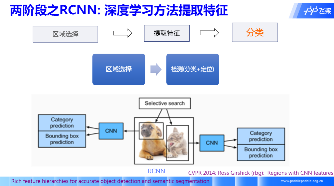
RCNN

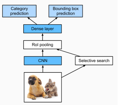
Fast-RCNN

• 引入RoI Pooling操作，解决重复特征提取问题
• 将分类和回归损失统一在同一个框架中
• 通过Selective Search提取候选框，速度慢，不是端到端

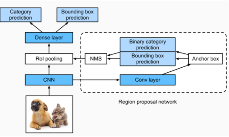
Faster-RCNN

• 通过RPN（Region Proposal Network）学习候选区域
• 提高了精度，速度快

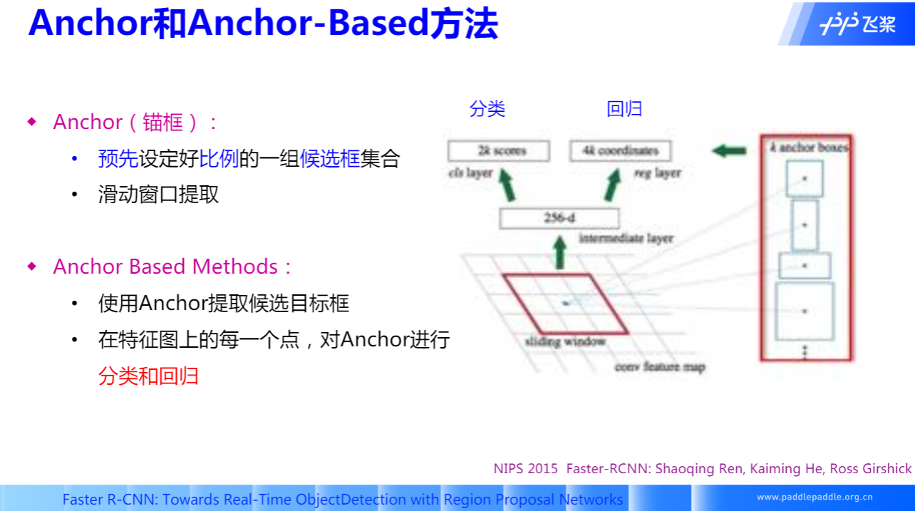
Anchor 和 Anchor-Based 方法

两阶段方法

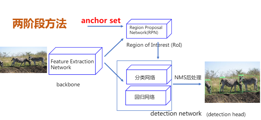
• 先使用Anchor回归候选目标框，划分前景和背景。
• 使用候选目标框进一步回归和分类，输出最终目标框和对应的类别
• R-CNN系列
  • RCNN、Fast-RCNN、FasterRCNN
  • FPN、CascadeRCNN、LibraRCNN……

一阶段方法

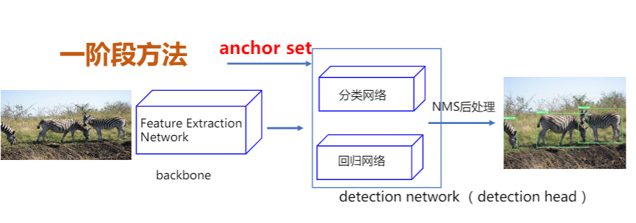
• 直接对Anchor回归和分类最终目标框和类别
• 算法：
  • YOLOv2 YOLOv3
  • SSD、RetinaNet

Anchor 缺点

• 手工设计
  • 数量？大小？长宽比？
• 数量多
  • 如何解决正负样本不均衡问题？
• 超参数
  • 如何对不同数据设置？

Anchor-Free 方法

不再使用预先设定的Anchor，通常通过预测目标的中心或者角点，对目标进行检测。

基于关键点的检测算法

先检测目标左上角和右下角点，再通过角点组合形成检测框。

基于多关键点联合表达的方法

• CornerNet/CornerNet-lite
• CenterNet: Keypoint Triplets for Object Detection
• RepPoints

基于中心的检测算法

直接检测物体的中心区域和边界信息，将分类和回归解耦为两个子网络。

基于中心区域预测方法：

• FCOS
• CenterNet: Objects as Points

三种算法对比

	Anchor-Based单阶段	Anchor-Based两阶段	Anchor-Free
网络结构	简单	复杂	简单
精度	优秀	更优秀	较优秀
预测速度	快	稍慢	快
超参数	较多	多	相对少
扩展性	一般	右边	较好

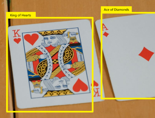
基本术语

BBox

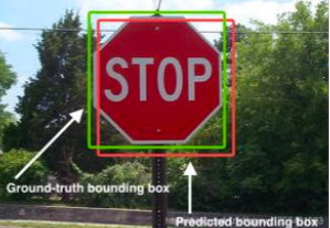
Bounding Box，边界框。

• 绿色为人工标注的ground-truth，红色为预测结果。
• 有两种表达形式：
  • xyxy：左上+右下
  • xywh：左上+宽高

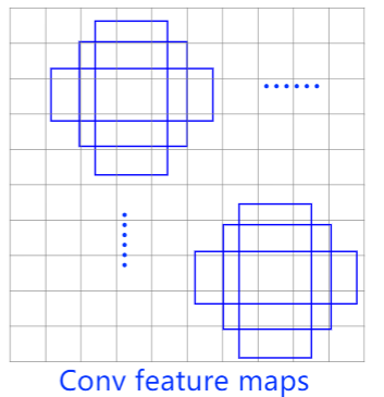
Anchor

锚框。

• 人为设定不同长宽比、面积的先验框。
• 在单阶段SSD检测算法中也被称为Prior Box。

RoI

Region of Interest，特定的感兴趣的区域。

Region Proposal

候选区域/框。

RPN

Region Proposal Network，在Anchor-Based的两阶段提取候选框的网络。

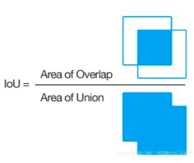
IoU

Intersaction over Union。交并比。
评价预测框的质量，IoU越大则预测框与标注越接近。

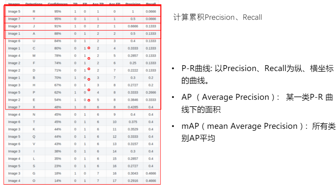
mAP

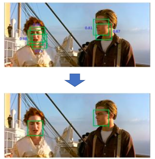
NMS^[3][4]

Non-Maximum Suppression，非极大值抑制。
目标检测的过程中在同一目标的位置上会产生大量的候选框，这些候选框相互之间可能会有重叠，此时我们需要利用非极大值抑制找到最佳的目标边界框，消除冗余的边界框。
非极大值抑制的流程如下：

• 根据置信度得分进行排序
• 选择置信度最高的比边界框添加到最终输出列表中，将其从边界框列表中删除
• 计算所有边界框的面积
• 计算置信度最高的边界框与其它候选框的IoU。
• 删除IoU大于阈值的边界框
• 重复上述过程，直至边界框列表为空。

#!/usr/bin/env python
#_*_ coding: utf-8 _*_


import cv2
import numpy as np


"""
    Non-max Suppression Algorithm

    @param list  Object candidate bounding boxes
    @param list  Confidence score of bounding boxes
    @param float IoU threshold

    @return Rest boxes after nms operation
"""
def nms(bounding_boxes, confidence_score, threshold):
    # If no bounding boxes, return empty list
    if len(bounding_boxes) == 0:
        return [], []

    # Bounding boxes
    boxes = np.array(bounding_boxes)

    # coordinates of bounding boxes
    start_x = boxes[:, 0]
    start_y = boxes[:, 1]
    end_x = boxes[:, 2]
    end_y = boxes[:, 3]

    # Confidence scores of bounding boxes
    score = np.array(confidence_score)

    # Picked bounding boxes
    picked_boxes = []
    picked_score = []

    # Compute areas of bounding boxes
    areas = (end_x - start_x + 1) * (end_y - start_y + 1)

    # Sort by confidence score of bounding boxes
    order = np.argsort(score)

    # Iterate bounding boxes
    while order.size > 0:
        # The index of largest confidence score
        index = order[-1]

        # Pick the bounding box with largest confidence score
        picked_boxes.append(bounding_boxes[index])
        picked_score.append(confidence_score[index])

        # Compute ordinates of intersection-over-union(IOU)
        x1 = np.maximum(start_x[index], start_x[order[:-1]])
        x2 = np.minimum(end_x[index], end_x[order[:-1]])
        y1 = np.maximum(start_y[index], start_y[order[:-1]])
        y2 = np.minimum(end_y[index], end_y[order[:-1]])

        # Compute areas of intersection-over-union
        w = np.maximum(0.0, x2 - x1 + 1)
        h = np.maximum(0.0, y2 - y1 + 1)
        intersection = w * h

        # Compute the ratio between intersection and union
        ratio = intersection / (areas[index] + areas[order[:-1]] - intersection)

        left = np.where(ratio < threshold)
        order = order[left]

    return picked_boxes, picked_score
#Image name
image_name = 'nms.jpg'

#Bounding boxes
bounding_boxes = [(187, 82, 337, 317), (150, 67, 305, 282), (246, 121, 368, 304)]
confidence_score = [0.9, 0.75, 0.8]

#Read image
image = cv2.imread(image_name)

#Copy image as original
org = image.copy()

#Draw parameters
font = cv2.FONT_HERSHEY_SIMPLEX
font_scale = 1
thickness = 2

#IoU threshold
threshold = 0.4

#Draw bounding boxes and confidence score
for (start_x, start_y, end_x, end_y), confidence in zip(bounding_boxes, confidence_score):
    (w, h), baseline = cv2.getTextSize(str(confidence), font, font_scale, thickness)
    cv2.rectangle(org, (start_x, start_y - (2 * baseline + 5)), (start_x + w, start_y), (0, 255, 255), -1)
    cv2.rectangle(org, (start_x, start_y), (end_x, end_y), (0, 255, 255), 2)
    cv2.putText(org, str(confidence), (start_x, start_y), font, font_scale, (0, 0, 0), thickness)

#Run non-max suppression algorithm
picked_boxes, picked_score = nms(bounding_boxes, confidence_score, threshold)

#Draw bounding boxes and confidence score after non-maximum supression
for (start_x, start_y, end_x, end_y), confidence in zip(picked_boxes, picked_score):
    (w, h), baseline = cv2.getTextSize(str(confidence), font, font_scale, thickness)
    cv2.rectangle(image, (start_x, start_y - (2 * baseline + 5)), (start_x + w, start_y), (0, 255, 255), -1)
    cv2.rectangle(image, (start_x, start_y), (end_x, end_y), (0, 255, 255), 2)
    cv2.putText(image, str(confidence), (start_x, start_y), font, font_scale, (0, 0, 0), thickness)

#Show image
cv2.imshow('Original', org)
cv2.imshow('NMS', image)
cv2.waitKey(0)

常用开源数据集

数据集	类别数	train图片数，box数	val图片数，box数	boxes/Image
Pascal VOC-2012	20	5717,13k+	5823,13k+	2.4
COCO	80	118287,40k+	5000,36k+	7.3
Object365	365	600k,9623k	38k,479k	16
OpenImages18	500	1643042,860k+	100000,696k+	7.0

---

1. 百度百科：https://baike.baidu.com/item/目标检测/8688936?fr=aladdin ↩︎

2. Zhengxia Zou, Zhenwei Shi, Yuhong Guo, Jieping Ye: “Object Detection in 20 Years: A Survey”, 2019; arXiv:1905.05055 ↩︎

3. 非极大值抑制(Non-Maximum Suppression), SnailTyan, https://www.jianshu.com/p/d452b5615850 ↩︎

4. Code: https://github.com/SnailTyan/deep-learning-tools/blob/master/nms.py ↩︎